INDIRECT function in Excel returns the reference specified by a text string. The syntax for this excel function is as follows.

Formula Syntax: INDIRECT( ref_text, [a1] )

ref_text can be the range of cells or a named range.

[a1] can be TRUE or FALSE. TRUE is used to indicate that ref_text is in R1C1 style and FALSE is used to indicate ref_text is in a1 style. If we omit this argument, it assumes ref_text to be in a1 style by default.

Indirect function when used with other functions like VLOOKUP and MATCH can be a very powerful function in excel.

INDIRECT function with VLOOKUP:

Let us take an example to know how INDIRECT function in excel works with VLOOKUP. We have total sales of products like Mobile and Laptop for different months in different sheets and we are interested in extracting that data month wise and find the total sales. To do this, we need to look up the sales values using VLOOKUP function with INDIRECT function.

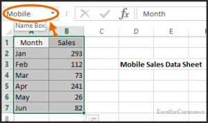
Step 1:  Creating named ranges

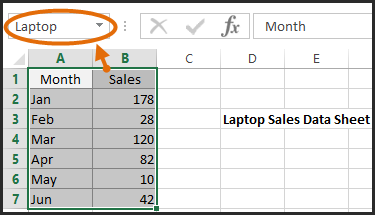
First, we need to name the ranges in the individual data sheets as Mobile and Laptop as shown in the image below.

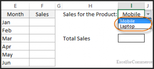
Step 2: Create Drop-down List

Now, back to the main sheet. Here we make a table in order to populate those monthly sales based on the dropdown list (Mobile or Laptop) in the cell (I1).

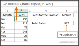
Step 3: Formula to extract the values

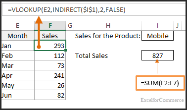
We use the formula “=VLOOKUP(E2,INDIRECT($I$1),2,FALSE)” in the Sales column (F). Here VLOOKUP (More about LOOK UP functions here) looks up the value in the cell E2, E3 and so on. The look-up table is found based on the INDIRECT function (I1). I1 is the dropdown list with the named ranges we named earlier. Based on these ranges in another sheet the INDIRECT function in excel redirects the required range references. Here ‘2’ in the formula is the column index number and we put FALSE as we are interested in extracting the exact value.

Now, if we want to get the total sales based on the drop-down selection, we can put the formula “=SUM(F2:F7)” in cell I7

This is how we look up values using INDIRECT function in excel combined with VLOOKUP function.

INDIRECT function with MATCH:

INDIRECT and Match functions when combined create a powerful tool to extract data. As we know by now that INDIRECT function pulls the required data from same/another sheet. What does MATCH do here? INDIRECT and MATCH function help in extracting three dimensional data. Let’s take an example to understand how it works.

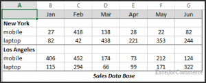
Assume that we have a Sales Data Base for months “Jan to Jun” for different cities/ areas and for different products (Mobile and Laptop) as shown in the image below. Here there are three criteria which are Area, Product and Total sales.

Step 1: Creating Calculation Column

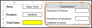
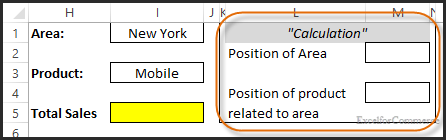
Now, we are interested in extracting the Total Sales for Area (I1) , for a product (I3) selected from the dropdown list. To do this, we need to create a calculation area (as shown in the image below) which helps to extract the data.

Note: We can hide the Calculation Column from user.

Step 2: Finding the Position of Area

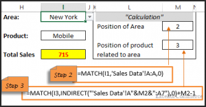
In this example we selected New York as Area and Product as Mobile. To know the row position of the Area selected we are using the formula “=MATCH(I1,’Sales Data’!A:A,0)” as shown in the image below.

We are using MATCH function, here look up value is ‘I1’ which is Area. Now we need to match this in the Sales Data sheet column A and put 0 at the end (as we need exact match). This formula will fetch the row number which is 2 in our example.

Step 3: Finding the Position of Product

Now based on the position of area we need to find the position of product which is related to that area. To find this we need to put the following formula

“=MATCH(I3,INDIRECT(“‘Sales Data’!A”&M2&”:A7″),0)+M2-1” as shown in the image above.

Here we are trying to get the actual position of Mobile by using the relative position of the area New York. To achieve this we are using Indirect function and Match function with lookup value I3 (‘Mobile’). For mentioning range we enter the sheet name as Sales Data and ‘A’ as column. We concatenate this with M2 (Position of Area i.e. 2) to get the range start A2 till A7 creating the range reference (“‘Sales Data’!A”&M2&”:A7″). The third argument 0 indicates we want an exact match. Now we have the relative position of the product that is Mobile for the Area ‘New York’. To get the actual position in the sheet, we need to add M2 (Position of area) and subtract 1 from the result to get the actual position of the product.

Step 4: Finding Total Sales

Now that we know the position of product, we can find the Total Sales by using the following formula. “=SUM(INDIRECT(“‘Sales Data’!B”&M4&”:G”&M4))”

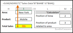
Here, we are using SUM function (to find total) with INDIRECT function (to extract the required range) on Sales Data sheet column B till G concatenating with cell M4 (Position of Product). Here Position of Product is the row number for the selected product. And the final result is 715 as total sales of Mobile in the city New York.

These are the two examples on how to use INDIRECT function in Excel to extract data from another sheet. Have queries? Feel free to contact our Excel Expert here.