Microsoft Excel is equipped with “What-If Analysis” tools like scenario manager, Goal-seek and Data table. These tools allow you to use different data sets in one or more formulas to come up with different sets of results.

For example, scenario manager can be used to compare two different budgets at the same time using its “Summary” option. The goal-seek in excel is helpful in allowing to predict the input values for a desired output value. So, basically “what-if analysis” allows a user to change the cell values in a spreadsheet to observe the outcomes of changes based on the formulas.

Scenario Manager

As mentioned earlier, Scenario manager in what-if analysis allows you to save “Scenarios” which are similar data sets with different values. Scenario manager is very helpful in comparing two or more business events.

Case Study:

• Let us take the example of annual sales of a company for two years before and after recession.
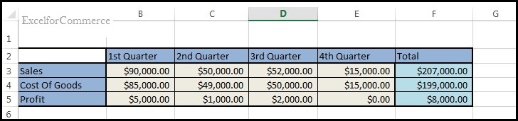
• The sales data of the company before recession is taken in a spreadsheet comprising Sales revenue, Cost of goods and Profit for four quarters in the year.

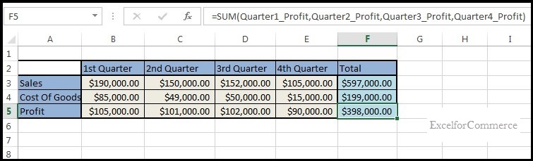
• The total value for Sales, Cost of goods and Profit is calculated in F3, F4 and F5 respectively.
• Each and every cell in the data which contains a value is given with a unique name in the names manager.

• Doing this will avoid the values being denoted as cell references in the final “Summary report” making it easier to understand.
• Now let us make use of “Scenario Manager” to create two different scenarios namely “After recession” and “Before Recession”.
• Select What-if analysis from the data tab and then select “Scenario Manager” from the menu.

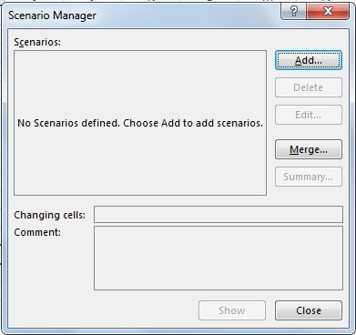
• Click on “Add” to add the scenario “Before Recession”

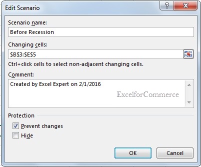
• The ‘Changing cells’ is given with the reference “B3:E5” which contain the sales, cost of goods and profit values.
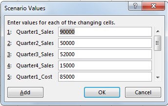
• On Clicking ‘OK’, the ‘Scenario Values’ box pops up containing values given in the ‘Changing cells’ section previously.

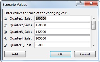
• Click “OK” upon verifying the values.

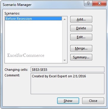
• You will notice that the “Before Recession” scenario is created successfully.

Now, the second scenario has to be added so that the values can be compared. For this, make the necessary changes to the same data to reflect after-recession values. Here, in our case, the Revenue values drop due to poor economic conditions after the recession. So, change the metrics accordingly.

• After entering the values into the respective cells, select the “scenario manager” again to add the “After recession” scenario.

• The ‘Edit Scenario’ box pops up. The changing cells will be given with the same reference which is given in the last scenario i.e. “B3:E5″.

• Click “OK”

• The scenario values box will now hold the new values given for this scenario. Click OK after verifying.

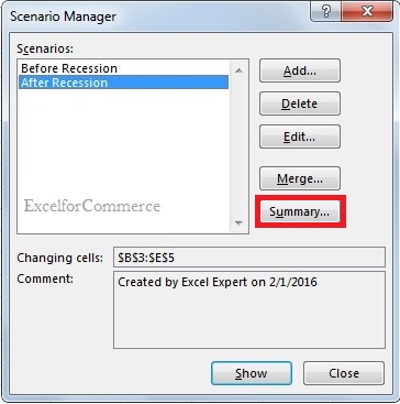
• Notice that both the scenarios are added to the scenario manager.
• This way, you can keep on adding as many scenarios for comparison.

     Our main objective here is to compare both the scenarios before and after recession.

• Select the “Summary” option in ‘Scenario Manager’ box.

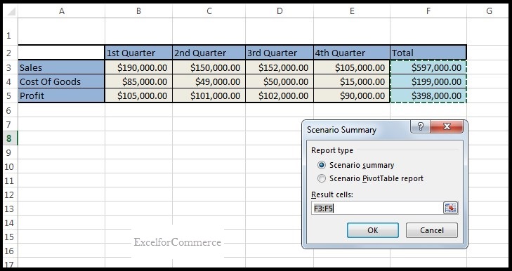
• Select “Scenario summary” option which enables you to compare both the scenarios added.
• In, “Result cells” enter the reference F3:F5 which hold the total sales, cost and profit. These will be included in the “Scenario summary” report.
• Click OK.

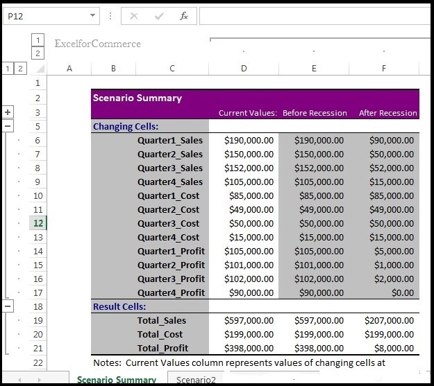
• You will see the Scenario summary report created in a new worksheet. As you can see, the drastic drop in the profits of the company after recession clearly indicates the economical slowdown caused by the recession.  The “Result Cells” clearly shows the difference between the “After Recession” and “Before Recession” values. The total profit value after recession ($8000) is just 2 % of total profit value before recession ($398,000) which is really a matter of concern for a company.

Comparing different scenarios using scenario manager is simple yet efficient. Even when scenarios to be compared are more in number, the summary derived from the scenarios can be easily analyzed.

Goal Seek

Goal-seek helps us find out or seek the initial input needed to get a desired output from a formula. Goal seek does trial and error to seek a goal abiding by the formula specified for the “target value” we want.

Case Study:

Let’s take the example of an electronics store, where the products fall into 3 different categories – Laptops, Mobiles and Tablets. The profit margins for Laptop, mobiles and tablets are 10%, 20% and 30% respectively. As you can see in the below screenshot, the product of revenue earned and the gross margin gives us the gross profit.

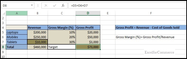
The “Revenue” column contains the revenue generated by laptops, mobiles and tablets. The total revenue is calculated as $460,000. The profit margin for each category of product is given individually in the “Gross margin” column.  The Gross profit column contains profit values for laptops, mobiles and tablets. The total profit is calculated in D8 as $73,000.

We are interested in knowing the following question

“By what amount should the tablet sales revenue in cell B7 be increased so that the total profit in the cell D8 sums up to $100,000?”

• To find out, select “Goal-seek” from what-if analysis in the data tab.

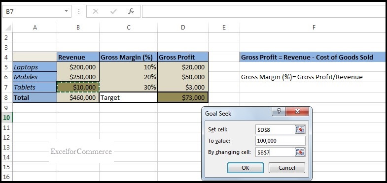
• The “Set cell” is given as G8 because we want to see how much the revenue generated by Tablets must be increased so that a value of $100,000 total gross profit is achieved.
• “To value” is given as $100,000 which is our target value. Our objective is to achieve the target value by changing the sales of tablets.
• Set “By changing cell” as B7 and click “OK”.

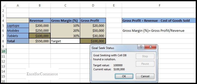
• The “Goal Seek Status” box displays the status of solution. Click “OK” once the answer is successfully found. Therefore, to get a total profit of $100,000, the revenue derived by sales of tablets must be increased to $100,000

This is how Goal seek in excel can be used to find out the inputs when you already know the target value to be achieved.

Data Table

Data table is used in calculating multiple results by following multiple constraints at a time. It helps in showing how the output values of one or more cells change, by changing one or more variables in the formula.  Data table enables you to calculate and compare values of different outputs derived from the same formula by giving varying inputs, all in one worksheet.

Case Study:

Let us suppose you want to compare home loan plans offered by different banks which lend the amount at different interest rates. You have applied for a loan for $2,000,000 in bank at 7% interest rate for a repayment period of 20 years. PMT formula is used to calculate the monthly payment which is derived as $15,506 in cell C7.

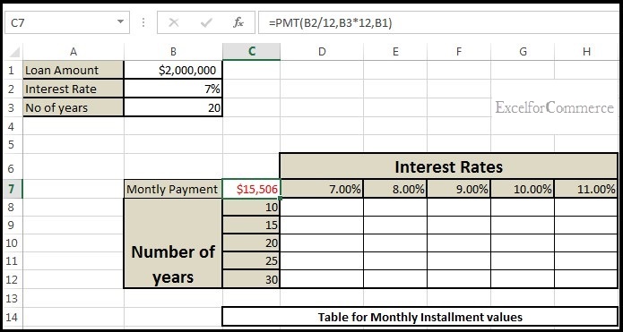
• The objective here is to derive the EMI values at different interest rates and different number of years for repayment. So, a table is created accordingly.

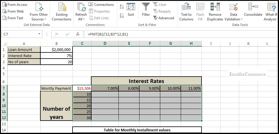
• Now, Select the cell range “C7:H12” and choose “data table” from what-if analysis menu. Doing this will enable “Data table” tool to understand the formula used to derive the EMI value in cell C7 and apply the same formula in calculating EMI values in the cells “D8:H12”.

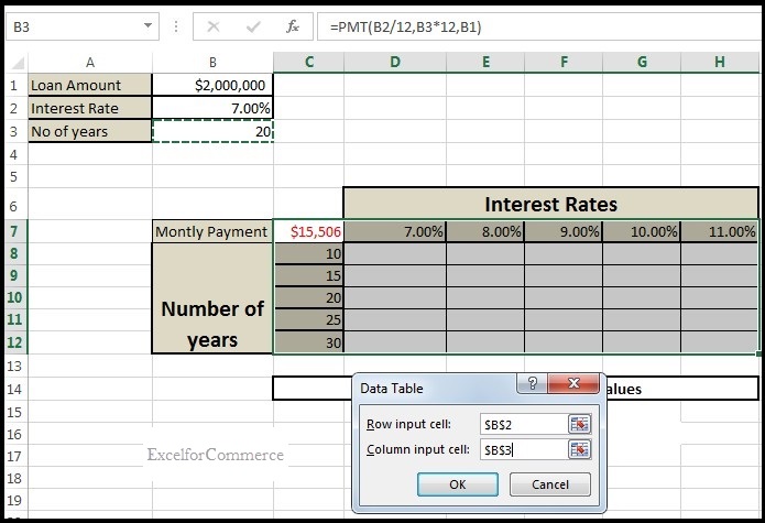
• In the Data Table box, the “Row input cell:” is given as B2 which holds the interest rates. Notice that the row values of the selected table are interest rates too.
• The “Column input cell:” is given with B3 which contains “Number of years” value. Also notice that column values of the table are “Number of years”. Click OK.

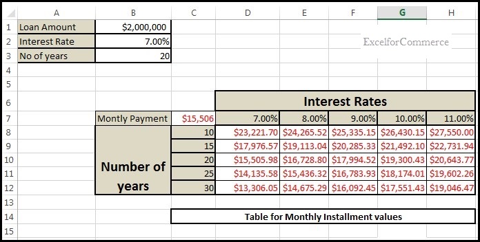
• Notice that the EMI values are calculated according to their respective “Interest rates” and “Number of years” values and written in their respective cells.
• The EMI for the loan taken at 8% interest rate with the repayment period of 20 years is $16728.80. The EMI for the loan taken at 11% interest rate for 30 years of repayment period is $19,046.47 and so on. In this way, data table makes it easy for us to find out multiple values for multiple constraints at a time, at one place.

The what-if analysis tools are very helpful to analyse your business scenarios and come up with solutions for many “what-if” problems in your day-to-day business cases. If you have any questions on what-if analysis, feel free to contact us at excelexpert@excelforcommerce.com.