The process of looking up specific values in a data set is the most common task in Excel. If your intent is to become an Excel Expert someday then you will need a good understanding of all the lookup formulas available in Microsoft Excel. There are 6 lookup functions in excel: LOOKUP, VLOOKUP, HLOOKUP, (INDEX & MATCH) and OFFSET.

Once we have a data repository in Excel, we may want to generate reports or extract meaningful information from it. That’s when the LOOKUP functions in excel can be useful. These lookup functions are explained in this blog, taken one at a time.

LOOKUP function in Excel:

The LOOKUP function returns a value either from one-row or one-column range or from an array. The LOOKUP function has two syntax forms: the vector form and the array form.
Formula Syntax: LOOKUP(lookup value, lookup range, [result range] )

Lookup value is the value which we want to lookup, lookup range is the range where we want to check whether our lookup value is present in the range, and result range is the range from where we want to extract the required information.

Let’s take an example, the sample data below contains information of few students with their respective marks and their results. We are interested in extracting the academic details which include Roll number, marks and the result. This task can be easily done using the LOOKUP function in excel.

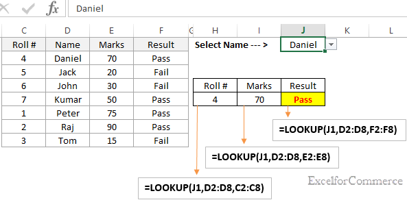
Let’s make a dropdown list with student names in the cell (J1) based on the student name selected from the dropdown, the corresponding output is shown in the range (H5:J5). Let see the formulas used to extract the desired information from the data table.

To extract Daniel’s Roll number we used the formula “=LOOKUP(J1,D2:D8,C2:C8)”. Here J1 is the Lookup value (name of the student), (D2:D8) is the Lookup range where we want to find the name of the student selected in cell J1 and (C2:C8) is the result range (roll number). The formula first identifies the position (row number) of the name selected (Daniel) in column D and displays the information from column C (roll number) for the same row number.

To extract Daniel’s Marks we used the formula “=LOOKUP(J1,D2:D8,E2:E8)”. Here J1 is the Lookup value (name of the student), (D2:D8) is the Lookup range where we want to find the name of the student selected in cell J1 and (E2:E8) is the result range (Marks). The formula first identifies the position (row number) of the name selected (Daniel) in column D and displays the information from column E (Marks) for the same row number.

Similarly, to extract Daniel’s result status we used formula “=LOOKUP(J1,D2:D8,F2:F8)”. Here J1 is the Lookup value (name of the student), (D2:D8) is the Lookup range where we want to find the name of the student selected in cell J1 and (C2:C8) is the result range, The formula first identifies the position (row number) of the name selected (Daniel) in column D and displays the information from column F (Result) for the same row number.

Advantage of LOOKUP function:

The advantage of Lookup function is that it also provides backward lookup (unlike Vlookup), as we can see in the above example, roll number (left most column or column C) was displayed based on the name (Daniel) selected (column D).

Drawback of LOOKUP function:

The main drawback of LOOKUP function is that, the LOOKUP value column (in our case column D) must be sorted in ascending order before using the LOOKUP function in excel.

VLOOKUP function in Excel:

VLOOKUP formula in Microsoft excel performs a vertical lookup by searching for a value in the left-most column of table array and returning the value in the same row in the index number position. Vlookup formula is one of the most used formulas in Excel.
Formula Syntax: VLOOKUP( lookup value, table array, column index number, [range lookup] )

In VLOOKUP, lookup value is the value which we want to lookup, table array is the table from where we are trying to extract the required data, column index number is the column number (starting from left most column) from which the required value is to be extracted, Range lookup is optional, Enter FALSE to find an exact match. This is used when you are interested in exact match in the table. Enter TRUE to find an approximate match, which means that if an exact match is not available, then the VLOOKUP function will look for the next largest value that is less than required value. By default, the VLOOKUP function returns an approximate match if it is left blank.

Let’s take an example, sample data below contains SKU codes of products and their location in the warehouse. We are interested in extracting the Item name and its location. This task can be easily done using the VLOOKUP function in excel.

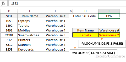
To extract Item Name, we use VLOOKUP formula as shown in the above image. “=VLOOKUP(I1,D2:F8,2,FALSE)”. Here I1 is the Lookup value ‘1392’ which we are trying to look in the table array of (D2:F8) with the index number being ‘2’ as we require Item name which is in the second column in the table array. We select FALSE as we need to find the exact match.

Similarly, to find Warehouse#, we use VLOOKUP formula as shown in the above image. “=VLOOKUP(I1,D2:F8,3,FALSE)”. Here I1 is the Lookup value ‘1392’ which we are trying to look in the table array (D2:F8) with the index number being ‘3’ as we require Warehouse # which is in the third column in the table array, We select FALSE as we need to find the exact match. Now, VLOOKUP looks for ‘1392’ from leftmost column and returns the warehouse number ‘Warehouse 2’.

So from the above example we can understand that VLOOKUP formula looks up from the leftmost column.

Advantage of VLOOKUP function in Excel:

The main advantage of this Excel function over LOOKUP function is that data in the table array need not be sorted.

Drawback of VLOOKUP function in Excel:

The only drawback is that, the lookup value should always be on the left most column of the table array.

HLOOKUP function in Excel:

HLOOKUP formula in Microsoft excel looks for a value in the top row of a table and returns the value in the same column from a row we specify.
Formula Syntax: HLOOKUP( lookup value, table array, row index number, [range lookup] )

Unlike VLOOKUP, HLOOKUP formula looks up horizontally. So, this function is preferred when we have a table array layout where all the headings are in one column. In HLOOKUP formula, lookup value is the value which we want to lookup, table array is the table from where are trying to extract the required data, row index number is the row number (starting from top most row) from which the required value is to be extracted, Range lookup is optional, Enter FALSE to find an exact match. This is preferred when you are interested in exact match in the table. Enter TRUE to find an approximate match, which means that if an exact match is not available, then the HLOOKUP function will look for the next largest value that is less than required value. . By default, the HLOOKUP function returns an approximate match if it is left blank.

Let’s take an example, sample data below contains the data of employees of a company where they received bonus on monthly basis. We are interested in extracting the Employee Name and his Bonus for the selected month from the dropdown list in the cell F5. This task can be easily done using the HLOOKUP function in excel.

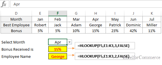
To extract Bonus Received, we use HLOOKUP formula as shown in the above image. “=HLOOKUP(F5,E1:K3,3,FALSE)”. Here F5 is the Lookup value ‘Apr’ which we are trying to look in the table array of (E1:K3) with the index number being ‘3’ as we require Bonus data from third row in the table array, We select FALSE as we need to find the exact match. Now, HLOOKUP looks for ‘Apr’ in topmost row and from the same column it returns the value ‘15%’ from the mentioned row index ‘3’.

Similarly, to extract Employee Name, we use HLOOKUP formula as shown in the above image. “=HLOOKUP(F5,E1:K3,2,FALSE)”. Here F5 is the Lookup value ‘Apr’ which we are trying to look in the table array of (E1:K3) with the index number being ‘2’ as we require Employee Name from second row in the table array, We select FALSE as we need to find the exact match. Now, HLOOKUP looks for ‘Apr’ in the topmost row and from the same column it returns the value ‘George’ from the mentioned row index ‘2’.

Advantage of HLOOKUP function in Excel:

The main advantage of this excel function is that data in the table array need not be sorted.

Drawback of HLOOKUP function in Excel:

The only drawback is that, the lookup value should always be on the topmost row of the table array.

OFFSET function in Excel:

OFFSET function in Microsoft excel returns a reference to a range that is a given number of rows and columns from a given reference.

Formula Syntax: OFFSET( reference, rows, columns,[height], [width] )

The reference is the starting range of the table, rows is the desired row number from the reference range, columns is the desired column number from the reference range, height is the number of rows which we need in the range and width is number of columns we need in the range.

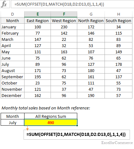
OFFSET function in Excel is most often used with other functions to get best out of it. Let’s take an example; we have a table with monthly sales in 4 regions (east, west, north and south). We are interested in finding monthly total sales of all regions. Say, we need to extract total sales for the month ‘July’ , to achieve this we use a formula “=SUM(OFFSET(D1,MATCH(D18,D2:D13,0),1,1,4))”

Let’s understand what MATCH function is as we are using it with OFFSET to MATCH and retrieve data. The Microsoft Excel MATCH function searches for a value in an array and returns the relative position of that item.

Formula Syntax:  MATCH(lookup value, lookup array, [match type] )

Here lookup value is the value which we are interested in matching it to the table, look up array is the range where are matching the lookup value and match type in most cases is 0 as we are looking for an exact match.

Now, coming back to the example, the month’s dropdown list is in the cell ‘D18’ where we select ‘July’. As we need SUM of total sales we start off with using SUM function (=SUM()), then to find the required range we use OFFSET, here D1 in the formula being the reference, Now let’s match the month ‘July’ from the Months column in the table (D2:D13) and as we need exact match we enter 0 after the lookup array of Match function, then columns is 1 as the column starts from the given reference, Height is 1 as our requirement is for one month which is July and width is 4, as we are interested in all four regions. In result, we sum the sales figures for the month July in the range (E8:H8) which turns out to be 490

INDEX AND MATCH in Excel:

INDEX function in Microsoft Excel returns either the value or the reference to a value from a table or range. This function has two syntaxes which are mentioned below.

Formula Syntax:  INDEX( array, row number, [column number] ) and

INDEX( reference, row number, [column number], [area number] )

The array is the range of cells or table, row number is the row number in the array, column number is optional, it is the desired column number from the array.

When INDEX function is combined with MATCH function then it becomes a very powerful lookup function in Microsoft Excel. We can use INDEX and MATCH functions to make a two way lookup in the table. Let us take an example to understand how this two way look up works using the INDEX and MATCH functions in Excel.

Consider, we have table where there are sales figures for products such as Mobiles, Laptops, and Tablets for a year. We are interested in finding the sales figures for Tablets for the month April. Here, we need to lookup both April and Tablets in the table to extract the required data. Hence it is a two way lookup.

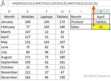
We select month April from the dropdown list in cell ‘J1’. We enter product name in the cell ‘J2’. We need to enter the following formula “=INDEX(E2:G13,MATCH(J1,D2:D13,0),MATCH(J2,E1:G1,0))” to obtain the result.

Let’s break the formula to understand and evaluate what the two excel functions are doing. Firstly, we used INDEX function with (E2:G13) as array, then we try to look up the month ‘April’ which is present in cell J1 using MATCH function. The lookup array here would be (D2:D13) and the third argument would be zero ‘0’ as we need an exact match. Now for matching the Product, we again use MATCH function with lookup value as ‘J2’ which is  ‘Tablets’ and lookup array (E1:G1) and zero as the third argument as we need exact match. This will return us the value 53 which corresponds to the month of ‘April’ and for Product ‘Tablets’.

These are the lookup functions in excel which are used based on the requirement to look up from the array of data. Still got doubts? CLICK HERE to contact our Excel Expert.