What is Monte Carlo Simulation?

The name Monte Carlo simulation comes from the computer simulations performed during the 1930’s to know the probability that the chain reaction needed for an atom bomb to detonate successfully. The physicists who involved in this work were big fans of gambling hence the name Monte Carlo.

How to use?

It is developed to analyze the problem by running the simulation many times in order to develop a statistical data on how the model works. The resulting data from the Monte Carlo simulation is close to the mathematical statistical probability. A problem with complexity is more efficiently solved using a Monte Carlo simulation.

In Excel, “RAND()” function is used to generate random values for Monte Carlo models. A new random real number is generated every time the worksheet is calculated, this is only possible when the Excel calculation are in Automatic. “RANDBETWEEN()” function is used to return a random integer number between the numbers we specify. Random numbers must be used to analyze output.

Example 1: Simulating coin toss using Monte Carlo Simulation

Let’s simulate a coin toss to determine the probability of the coin resulting in heads or tails. We will repeat the simple coin toss many times and then we calculate the percentage of heads.

Step 1: Creating a table

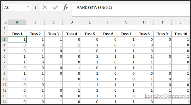
Lets create a table with 10 tosses being generated randomly using “=RANDBETWEEN(0,1)” function as shown in the image below. A ‘zero’ mean tails while ‘one’ means heads.

Here, we are generating a random sequence of integers between 0 and 1. Let’s populate the same formula for say 1000 simulations as shown in the image below.

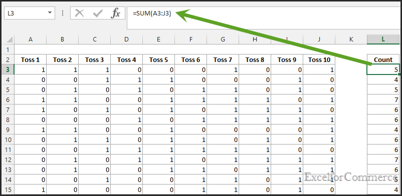
Step 2: Finding the count of Heads

To do this lets create a new column and put this formula. This will sum all the heads up (all 1’s) count

“=SUM(A3:J3)”

Step 3: Finding the Probability

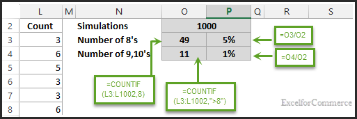
Now let’s find the probability of the Heads coming 8 times out of 10 tosses.

• In cell “O2”, we put the total number of simulations that we are running.
• In cell “O3”, we put the formula “=COUNTIF(L3:L1002,8)”

The above formula will help us find how many times that 8 out of 10 tosses gives heads

• In cell “O4”, we put the formula “=COUNTIF(L3:L1002,”>8″)”

This formula will help us find how many times coin turned heads in more than 8 out of 10 tosses

• In cell “P3”, we put the formula “=O3/O2”. This will give us the percentage of the count of heads falling 8 times.

• In cell “P4”, we put the formula “=O4/O2”. This tell us the percentage of the count of heads greater than 8 times.
• Hit ‘F9’ to generate random values and simulate the Monte Carlo Simulation.

Example 2: Predicting Sales based on Monte Carlo Simulation

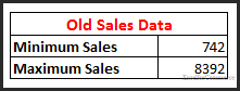
In this example, let’s assume that we have old sales data with an average, minimum and maximum sales for a period of 10 years and we are interested in finding the statistical data on how sales will turn out based on Monte Carlo Simulation.

Step 1: Generating data table

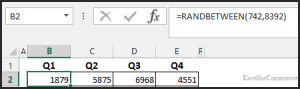
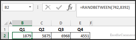
We generate random values based on our old min and max sales data as shown in the image below

“=RANDBETWEEN(742,8392)”

This will generate random values between 742 and 8392. These are generated for Q1, Q2, Q3 and Q4.

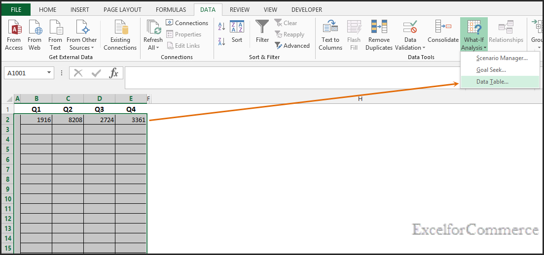
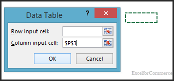
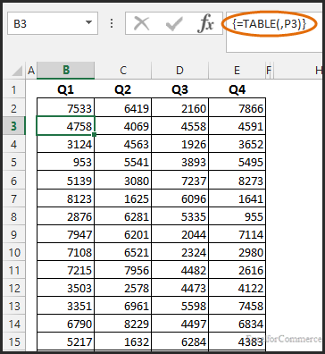
Now, let’s generate a data table with these random values. Select the whole table with an extra column as shown in the image below and click on Data Table present in What if analysis in Data Section in excel ribbon.

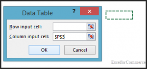
After clicking Data Table, we get a pop window where we need to enter the column input cell. Select some empty cell to allow excel perform its calculations.

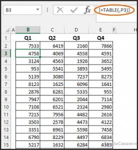
As shown in the image above, the data table has been generated.

Step 2: Calculating the Minimum, Maximum and Average

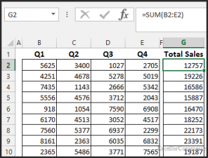
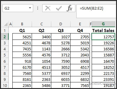
Create a total sales column “=SUM(B2:E2)”

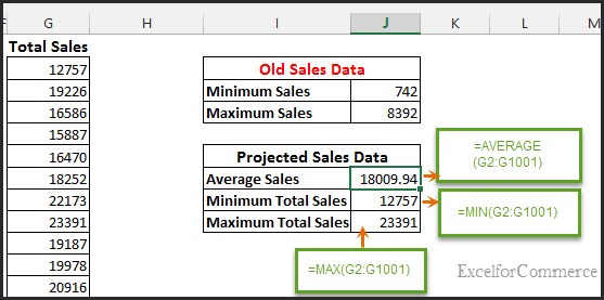
Based on 1000 simulations we find the Average, Minimum and Maximum total sales for our projected sales data as shown in the image above. By this data we can predict that Average sales and other details for a company.

Example 3: Creating Monte Carlo Simulation using Data Tables

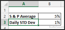
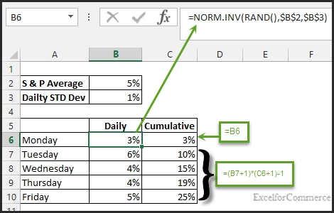
Let’s see how we can create Monte Carlo Simulation using Data Tables. We have ‘S & P Average’ (Stock Market Index) and ‘Daily STD Deviation’ over the past 10 years as shown in the image below.  We are interested in generating ‘1000’ simulated data of S & P and find the average, STD deviation and the probability of getting more than 30 % S&P at the end of the week.

Step 1: Let’s create Daily and Cumulative values

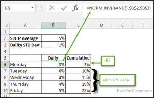
We generate ‘Daily’ values by using formula “=NORM.INV(RAND(),$B$2,$B$3)”

NORMINV is a statistical function. It returns the inverse of the normal cumulative distribution for the specified mean and standard deviation. For the probability argument we are using random function and for mean we are taking S&P Average cell ‘B2’ and for STD DEV we are taking Daily STD DEV cell ‘ B3’. Now populate the formula for remaining days.

For Cumulative, Monday will be same as ‘=B6’ and other is as shown below

‘=(B7+1)*(C6+1)-1’

Populate the same formula for remaining days in a week.

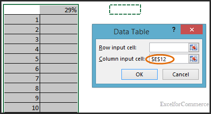
Step 2: Generate simulations using data table.

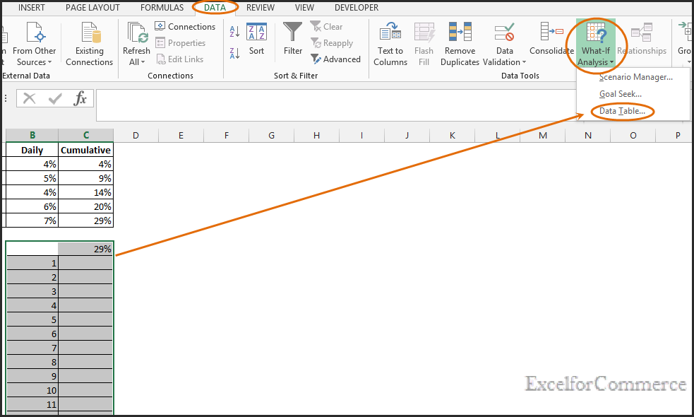
Select the table (first row in the table is having 29% which is the end of the week cumulative value) and click on Data Section in excel ribbon and then click on What if analysis and select Data table as shown in the image below

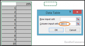
After clicking Data Table we get a pop window where we need to enter the column input cell, some empty cell away from data table has to be entered to allow excel perform its calculations.

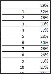
Based on the end of the week cumulative value the data table is generated as shown in the image below

Step 3: Finding Average, Standard deviation and Probability

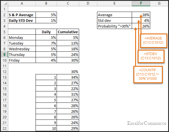
To find the Average for the simulated values we use the formula “=AVERAGE(C13:C1012)” and for STD Dev we use “=STDEV(C13:C1012)” and for Probability put the formula “=COUNTIF(C13:C1012,”>30%”)/1000”

There is 26% chance of getting more than 30% of S&P at the end of the week.

Have any Queries? Feel free to contact us here