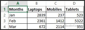
Dynamic charts in excel are useful when we add new data to our existing data tables. For example, lets take 1st quarter sales data for Laptops, Mobiles and Tablets as shown in the image below. A chart for such a data table is generally static i.e. the chart does not reflect new data which gets added to the existing data table. This blog will help you to create a dynamic chart which reflects new data points as and when new data gets added to the data table. To create dynamic charts we use offset function.

Step 1: Define a Named Range

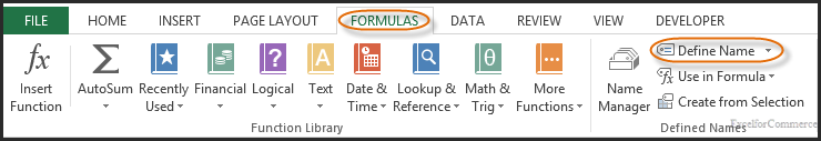
Step 1a:

To define a name range, select ‘Define Name’  in ‘Defined Names’ section in ‘Formulas’ tab in Excel ribbon.

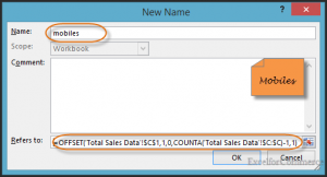
Step 1b:

A new window for defining a new named range will pop up. Here, we define the new name for our data ranges.

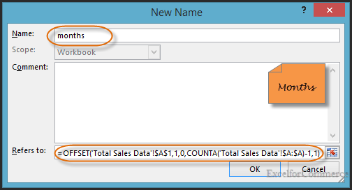
For Months, we enter Name as ‘months’ and put the following formula

“=OFFSET(‘Total Sales Data’!$A$1,1,0,COUNTA(‘Total Sales Data’!$A:$A)-1,1)”

Here, we use offset function. Offset function has five arguments:

1) ‘Total Sales Data’!$A$1: This is the reference cell. We are using A1 as starting reference because ‘Months’ column starts from this cell (refer to our sample data image).

2) ‘1’: This is the # rows from reference cell from which, our named range starts ($A$1 is our reference cell, since number of rows from reference cell is 1, our range ‘months’ starts from row # 2).

3) ‘0’: This is the # columns from reference cell from which, our named range starts (since reference cell is in column A and our range ‘ months’ is also in column A, the value is 0)

4) ‘COUNTA(‘Total Sales Data’!$A:$A)-1′: We use ‘COUNTA’ function to find the height (# used rows) of the range. We subtract 1 from the total range as we are using headers in our data table.

5) ‘1’: We end the offset function with 1 as width. Since our named range is only one column, width is 1.

Similarly, we define named ranges for Laptops, Mobiles and Tablets as shown in the image below.

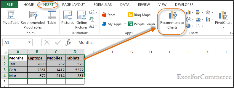
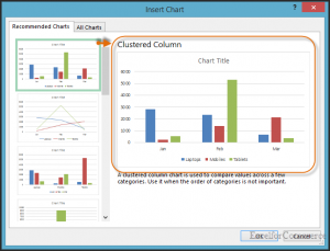
Step 2: Create a Chart

After defining named ranges, we select the data range and click on ‘Insert’ & then select the chart in ‘Charts’ area (Clustered bar chart in this example) as shown in the image below.

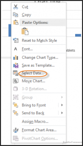
Step 3: Inserting Named Ranges into the chart (Dynamic chart in Excel)

To insert named ranges, we right click on chart and select  ‘select data’ option as shown in the image below.

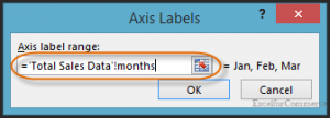
To make ‘months’ dynamic:

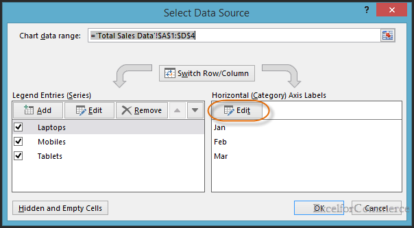
We click on Edit button to make changes for the month as shown in the image below.

Now, we get a pop up window (Axis Labels). Here instead of fixed range, we change it into named range (months).

To make ‘Laptops’ range dynamic:

Step 3a:

We click on Laptops

Step 3b:

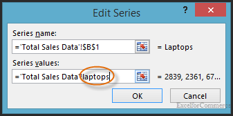
Now, we click on Edit as shown in the image below.

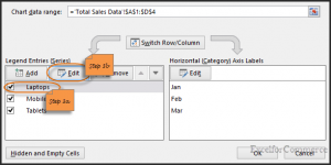
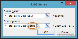
Now, we change the ‘series values’ (range) to our named range laptops

Similarly, we edit the data range for mobiles and tablets.

Steps above would help us in creating dynamic charts in excel. If you still have any questions, feel free to contact us here.