An Array formula works with an array. You may see array formulas referred to as “CSE formulas,” because you press CTRL+SHIFT+ENTER to enter them into your workbooks.

The following is a list of functions in Excel that use arrays:

1. LINEST()
2. MDETERM()
3. MINVERSE()
4. MMULT()
5. SUM(IF())
6. SUMPRODUCT()
7. TRANSPOSE()
8. TREND()

In general, array is a collection of items or values. An array formula is a formula that can perform multiple calculations on one or more of the items in an array. They can return either multiple results or a single result. An array formula that resides in multiple cells is a multi-cell formula, and an array formula that resides in a single cell is a single-cell formula, typically using SUM, AVERAGE, or COUNT, to return a single value into a single cell. Array formula will speed up creating formulas by eliminating unnecessary calculations. Array formulas are considered as a powerful tool in Microsoft Excel.

Example 1: How to Transpose using an array formula.

In general we know how to use Transpose by ‘Paste Special Transpose’ option to switch rows to columns or columns to rows. You can also use the TRANSPOSE function to achieve this. But here, we use array to do the transpose with a nifty feature which helps to link the Transposed data with the main table (Available for older versions of Excel only and not available in office 365).

Assume that we have data which is laid out in Columns and now we are interested in having it in Rows as shown in the image below.

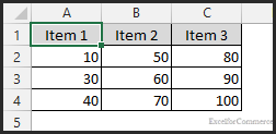
To do that, now let’s create a table with 4 columns and 3 rows to accommodate the data.

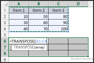
Now, select the whole table and put the Transpose function as shown in image below. As this is an array function we need to press CTRL+SHIFT+ENTER (CSE) instead of just hitting enter. Array function will not work unless we use “CSE”.

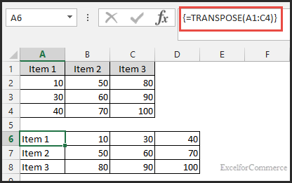
Now the table is generated as shown in the image below. As we can see in the formula that the Transpose function is enclosed in the curly braces indicating that it’s an array function.

We cannot delete the data from a single cell or delete a row from the newly generated table as it is an array and it will show the following message when a user does it.

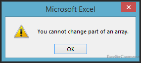
To delete the data and redo it, you need to select the whole range and delete all the data in the second table.

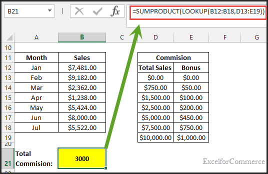
Example 2: Let’s see how we can derive Commission for a sales person

Assume we have a sales person and we have a table of data with sales figures as shown in the image below. We are interested in finding his commission without much of a calculations. To achieve this we use array in Look up function.

To calculate Total Commission we use Sum Product with Lookup function. Lookup function can deal with arrays.

=SUMPRODUCT(LOOKUP(B12:B18,D13:E19))

Here Lookup value is B12:B18 which are sales figures from Jan to Jul.  D13:E19 is the look up array and sum product returns the sum of the products of arrays. This results in $3000 as his Total Commission.

Points we need to remember while using Array Formulas:

1. Use arrays of equal size.
2. To create an array formula you need to hit CTRL+SHIFT+ENTER
3. We cannot edit Individual cells if they are in the array
4. Rows/Columns cannot be deleted if they are in the array.
5. Array calculations are limited based on the available memory on computer.
6. Too many array formulas will slow down recalculation.

Have any Queries? Feel free to contact us here