Dynamic dropdown list in Excel:

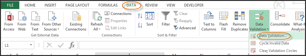
Dynamic dropdown list in excel falls under Data Validation. This can be accessible in Data Tools section in Data tab in excel ribbon as shown in the image below. Data Validation picks from a list of rules to limit the type of data that can be entered in a cell. dynamic dropdown list will limit the choices by using the named ranges and we need to use INDIRECT function to create the list.

Let’s take an example, we have a data of products (like mobile, laptop etc.) with their model numbers. We are interested in creating a dynamic dropdown list of model numbers based on the product selected. If we select Mobile from the products, then the dependent model numbers of mobile are shown in the dropdown list. Similarly, if we select Laptop from the products, then the dependent model numbers of laptops are shown in the dropdown list.

Let us go through the steps for creating a dynamic dropdown list in excel.

Step 1: Creating list of data

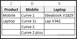
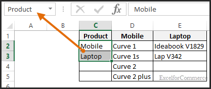
We first create the list of products and their model numbers in separate columns in same sheet or another sheet as shown in the image below. ‘Column C’ contains the Products list, ‘Column D’ contains the Mobile model numbers and ‘Column E’ contains the Laptop model numbers.

Step 2: Defining Names to the list

Now we name these lists as to create named ranges which are later used in the dynamic dropdown list in excel. Select the range C2:C3 and name it as ‘Product’ shown in the image below. Similarly, we name select D2:D5 and name it as ‘Mobile’ and select E1:E2 and name it as ‘Laptop’

Step 3: Creating Data Validation

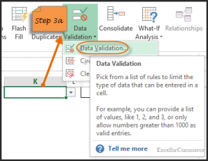
Step 3a:

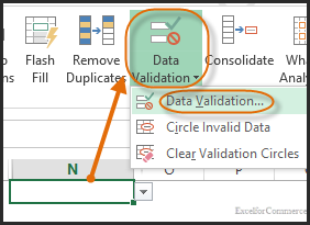
Now we go to the cell (K1) where we are interested in creating the dynamic dropdown list. Here we click on Data Validation and select Data Validation from the list.

Step 3b:

Now we get a pop-up window as shown in the image below.

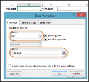
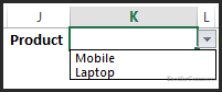
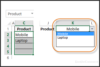
We select List in the Allow selection and we enter ‘=Product’ (named range) as the source and then click OK. Now we can see that the dropdown is showing the product list.

Step 4: Creating Dynamic Dropdown list in Excel

Step 4a:

Now we create a dynamic list based on the selected product name. Click on the desired cell say N1 and click data validation as shown in the image below.

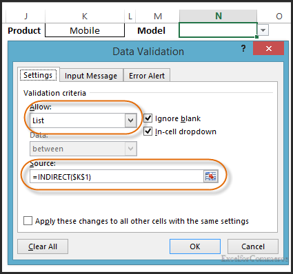
Step 4b:

After clicking on Data Validation we get a settings window. Here, we select List in the Allow selection and put “=INDIRECT($K$1)” and then click OK as shown in the image below.

The INDIRECT function here returns the reference list specified by the value in the cell (K1).

The Final output is as shown in the image below.

Dynamic Dropdown list in Excel excluding blank cells:

When we create a dropdown list at times we want to add more values to the list later. If we have a list of 3 items and we want to add another three somewhere in future. To create such dropdown, we select extra cell beforehand (C2:C5) but this will add blanks in the dropdown list as shown in the image below.

To overcome this, we generally select Ignore blanks while creating the dropdown list but this doesn’t help. We need to create a dynamic dropdown. To do this we first create a named range using OFFSET and COUNTA function.

Step 1: Defining Name in Name Manager

Step 1a:

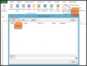
Select Name Manager in Defined Names section in FORMULAS tab

Step 1b:

Click New Name as shown in the image below.

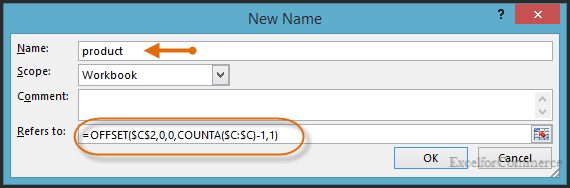
Step 2: Creating New Name using a Formula

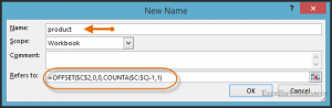
We now enter the name and put a formula “=OFFSET($C$2,0,0,COUNTA($C:$C)-1,1)” and then click OK. OFFSET will return a range based on a Starting position, the Row offset, the Column offset, the Height (number of rows down) and the Width(number of columns). COUNTA counts the number of non-blank cells. So, we count the number of non-blank cells in a row and use that as the Height for OFFSET.

Step 3: Creating Dropdown

Step 3a:

Now create dropdown, Select cell (K1) and click on Data Validation and select Data Validation

Step 3b:

Now, we get a pop-up window. We select List in the Allow selection and we enter ‘=Product’ (The new named range which we created using OFFSET AND COUNTA formula) as the source and then click OK as shown in the image below.

Now the dropdown list is dynamic. If we want to add new items/ values then we can add and this automatically get reflected in the dropdown list.

The drawback in using this COUNTA function is that, if there are any blank cells in between your range then COUNTA number will be wrong. Because the non-blank cells are not counted resulting in shorter range and the last cells in that range will be skipped.

This is how we create a dynamic dropdown list in excel and dynamic dropdown list excluding blank cells. Still got queries? Contact our Excel Expert here.