
- 11Nov2014
-
How to apply Conditional formatting in Excel?
Conditional formatting in Excel is used to highlight a cell or value/text in the cell, when certain conditions are met. Conditional Formatting can quickly spot trends and patterns in your data with bars, colors and icons by visually highlights important values.
Conditional formatting is based on the cell rules we amend. We can do a whole lot of things with this type of formatting. Pre-defined rules are available to select from the list to be used in general. But, at times only the built in formatting rules are not sufficient. So, we add our own formula to the conditional formatting taking the formatting to a whole new level. This blog is to give you a brief overview of conditional formatting with few examples for better understanding.
Where can I see conditional Formatting in Excel menu bar?
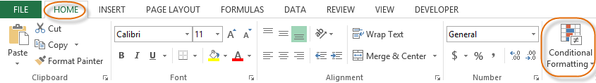
To access Conditional Formatting, Select HOME in the ribbon –> click Conditional Formatting to view the available preformats.
There are a lot of Preformats that Excel provides us. Let us discuss them one by one.
1) Highlight cell rules (Highlighting all cells which are more than a particular number):
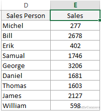
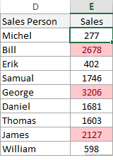
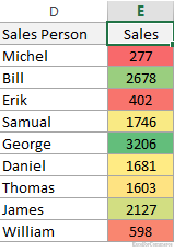
Let’s take a simple example of sales persons with their sales figures to illustrate conditional formatting in excel. We are interested in finding the sales figures which are more than 2000 in the given set of data. Let’s see how the predefined rules are applied to this particular example.
Step 1: Selecting conditional formatting
Step 1a:
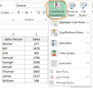
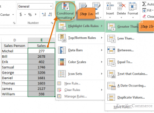
To apply conditional formatting, select the range (E2:E10) and click condition formatting in the excel ribbon and select Highlight Cell Rules
Step 1b:
Select ‘Greater than’ as we are interested in finding the sales figure greater than 2000.
Step 2: Applying Rule
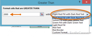
Enter 2000 and select how we want to fill the cell color as shown in the image below and click OK.
As we can see that the cells having the values which are greater than 2000 are highlighted as shown in the image below.
There are many other similar options in ‘Highlight Cell Rules’ like ‘less than’, ‘between’ or ‘equal to’ a value. Another two rules that come under this category are ‘Date occurring’ and ‘duplicate values’.
2) Top/Bottom Rules (Highlighting all cells which are top 10):
These rules are used to highlight Top 10 values or percentages and Bottom 10 values or percentages in a data list. These are also used to highlight above average and below average values.
Let’s take the same example of sales persons with their sales figures to illustrate this conditional formatting pre-format.
Step 1: Selecting Conditional Formatting
Step a:
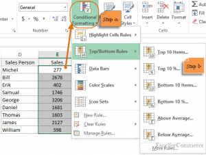
To apply conditional formatting, select the range (E2:E10) and click condition formatting in the excel ribbon.
Step b:
Select Top/ bottom Rules then select ‘Top 10’ as we are interested in top 3 sales figures in our data.
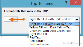
Step 2: Applying Rule
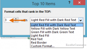
Enter 3 (as we are interested in selecting top 3) and select how we want to fill the cell color as shown in the image below and click OK.
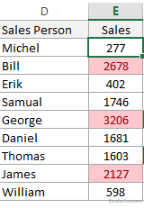
The highlighted cells are top 3 sales numbers as shown in the image below.
There are many others similar options in ‘Top/ Bottom Rules’ like Bottom 10, Top and Bottom 10% and above and below average.
3) Data Bars (Highlight all cells based on their values):
Data Bars are of two types – Gradient Fill and Solid Fill type. These are used to fill the cell based on its value. The higher the value, the longer the bar inside the cell. Let’s apply this type of conditional formatting to our sample data.
Let’s take the same example of sales persons with their sales figures to illustrate Data Bars in conditional formatting.
Step 1: Applying Conditional Formatting
Step a:
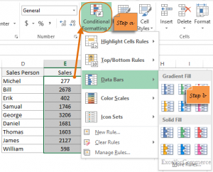
To apply conditional formatting, select the range (E2:E10) and click condition formatting in the excel ribbon and select Data Bars
Step b:
Select ‘Gradient fill’ or any other as per requirement.
After selecting the gradient fill the final output will be as shown in the image below.
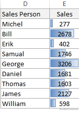
From the above example we can see that sales figure ‘3206’ of employee George has the longest data bar covering the entire cell as this value is the highest.
4) Color Scales (Highlight all cells based on their values):
These are RGB scales. These are used to apply a color gradient to a range of cells. The color indicates where each cell values falls in the given range.
Let’s take the same example of sales persons with their sales figures to illustrate Color Scales in conditional formatting.
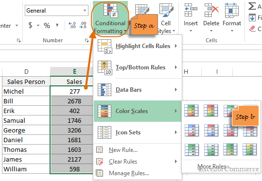
Step 1: Applying Conditional Formatting
Step a:
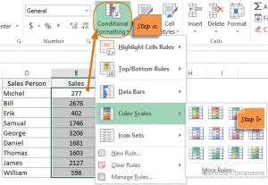
To apply conditional formatting, select the range (E2:E10) and click conditional formatting in the excel ribbon and select Color Scales
Step b:
Now select the shade as per requirement.
Based on the color scale selection the output shade is applied. The final output image is as shown below.
Here Red indicates the value is low or below average in the whole set of selected data, Yellow indicates that the values falls in the average and Green indicates that the values are above average to the highest values in the selected set of data range.
5) Icon Sets (Add icons to the cells based on their values):
Choose an icon set to represent the value in the selected cells. Let’s go back to our example of sales persons with their sales figures to illustrate Icon Sets in conditional formatting.
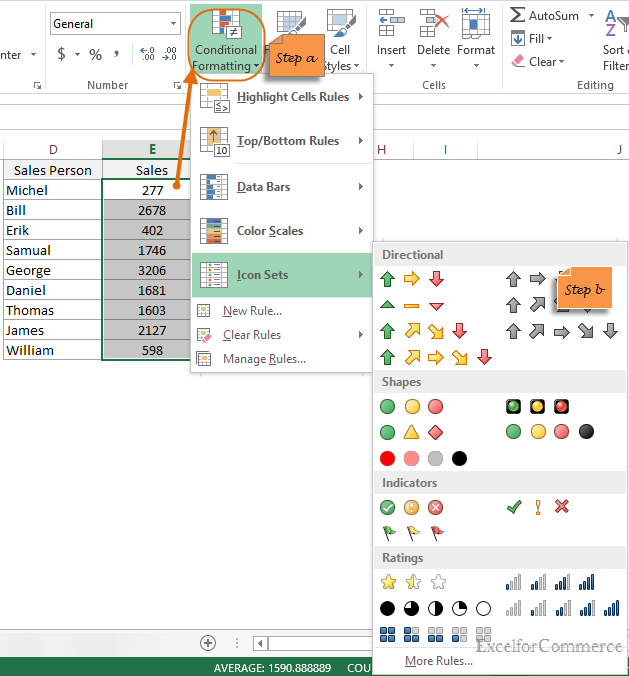
Step 1: Applying Conditional Formatting
Step a:
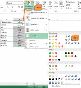
To apply conditional formatting, select the range (E2:E10) and click condition formatting in the excel ribbon.
Step b:
Select Icon Sets then select the icon shape as per requirement as shown in the image below.
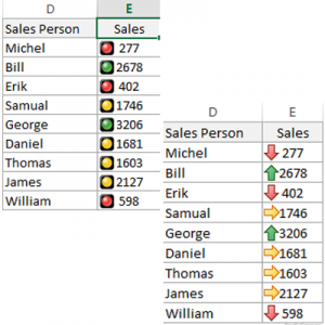
The final output image after applying the icon sets is as shown in the image below.
Icon sets has got a lot of options, we need to select those options based on our requirement. They are usually used when you want to format a metric like sales of a company, expenses of a firm showing a change or increase/decrease for a selected period.
In the above image we have selected Arrows to show whether the sales value is high or Low. These icons can also be used for representing stock values. Similarly we used a traffic light pattern where we can see the low numbered values are in red, medium range values are in yellow and High numbered values are in green.
6) Adding our own formula in conditional formatting
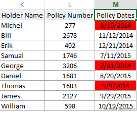
In order to add our formula in conditional formatting we need to follow few steps. Let us take an example and check how the conditional formatting on a formula will work. Assume we have a data consisting of Policy holder name, Policy number and Policy dates as shown in the image below.
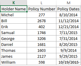
We are interested in finding the expiry date of the policies from today (Current date). Instead of going through row by row in the data manually, we can use conditional formatting to flag the expired policy cells with red fill.
Step 1: Selecting Conditional Formatting
Step 1a:
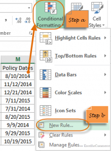
Select the range (M2:M10) and click condition formatting in the excel ribbon.
Step 1b:
Select New Rule from the following options.
Step 2: Formatting Rule
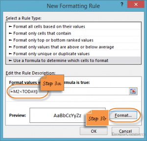
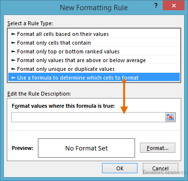
Now in new window for formatting rule select ‘Use a formula to determine which cell to format’ as shown in the image below. The formatting works when the formula returns TRUE.

Step 3: Entering formula
Step 3a:
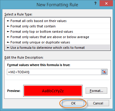
We put the following formula “=M2<TODAY()” as shown in the image below.
Step 3b:
After we enter formula, we click FORMAT button
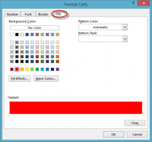
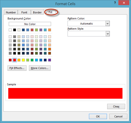
In format cells window go to fill tab and fill it with desired color. In this case we selected RED as fill color and click OK
Step 4:
After selecting the fill color, we return to formatting rule window, here we need to click OK to apply the conditional formatting to the selected range of cells.

From the image below now we can consider that there are three expired policies.
These are few of the examples on how to use Conditional Formatting in Excel. If you still have any queries, contact our Excel Expert here.


- 11 Nov, 2014
- Excel for Commerce
- 0 Comments
- Conditional formatting in Excel, Excel Consultant, Excel Expert,
Comments